


We’ve all heard the old saying, You can’t add apples and oranges (Fig. 7–3).
This is actually a simplified expression of a far more global and fundamental
mathematical law for equations, the law of dimensional homogeneity,
stated as
Every additive term in an equation must have the same dimensions.
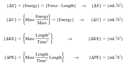
Consider, for example, the change in total energy of a simple compressible
closed system from one state and/or time (1) to another (2), as illustrated in
Fig. 7–4. The change in total energy of the system ( E) is given by Change of total energy of a system:
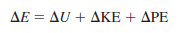
where E has three components: internal energy (U), kinetic energy (KE), and potential energy (PE). These components can be written in terms of the system mass (m); measurable quantities and thermodynamic properties at each of the two states, such as speed (V), elevation (z), and specific internal
energy (u); and the known gravitational acceleration constant (g),
m2/s2, all of which are equivalent. Suppose, however, that kJ were used in place of J for one of the terms. This term would be off by a factor of 1000 compared to the other terms. It is wise to write out all units when performing mathematical calculations in order to avoid such errors.
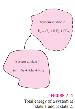
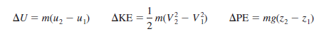
SOLUTION We are to verify that the primary dimensions of each additive term in Eq. 1 are the same, and we are to determine the dimensions of constant C.
Analysis (a) Each term is written in terms of primary dimensions,
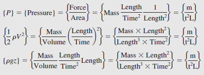
Indeed, all three additive terms have the same dimensions. (b) From the law of dimensional homogeneity, the constant must have the same dimensions as the other additive terms in the equation. Thus,
Primary dimensions of the Bernoulli constant: 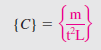
others, it would indicate that an error was made somewhere in the analysis.
Nondimensionalization of Equations The law of dimensional homogeneity guarantees that every additive term in an equation has the same dimensions. It follows that if we divide each term in the equation by a collection of variables and constants whose product has those same dimensions, the equation is rendered nondimensional (Fig.). If, in addition, the nondimensional terms in the equation are of order unity, the equation is called normalized. Normalization is thus more restrictive than nondimensionalization, even though the two terms are sometimes (incorrectly) used interchangeably. Each term in a nondimensional equation is dimensionless. In the process of nondimensionalizing an equation of motion, nondimensional parameters often appear—most of which are named after a notable scientist or engineer (e.g., the Reynolds number and the Froude number). This process is referred to by some authors as inspectional analysis.
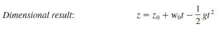
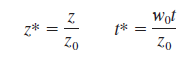
The constant and the exponent 2 in Eq. are dimensionless results of the integration. Such constants are called pure constants. Other common examples of pure constants are p and e. To nondimensionalize Eq. we need to select scaling parameters, based on the primary dimensions contained in the original equation. In fluid flow problems there are typically at least three scaling parameters, e.g., L, V, and P0 P , since there are at least three primary dimensions in the general problem (e.g., mass, length, and time). In the case of the falling object being discussed here, there are only two primary dimensions, length and time, and thus we are limited to selecting only two scaling parameters. We have some options in the selection of the scaling parameters since we have three available dimensional constants g, z0, and w0. We choose z0 and w0. You are invited to repeat the analysis with g and z0 and/or with g and w0. With these two chosen scaling parameters we nondimensionalize the dimensional variables z and t. The first step is to list the primary dimensions of all dimensional variables and dimensional constants in the problem, Primary dimensions of all parameters:

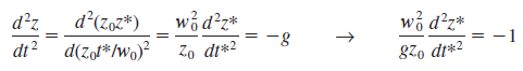
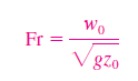
which is the desired nondimensional equation. The grouping of dimensional constants in Eq. 7–7 is the square of a well-known nondimensional parameter or dimensionless group called the Froude number,
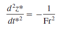
Nondimensional result:
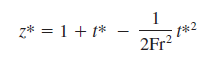
There are two key advantages of nondimensionalization . First, it increases our insight about the relationships between key parameters. Equation 8 reveals, for example, that doubling w0 has the same effect as decreasing z0 by a factor of 4. Second, it reduces the number of parameters in the problem. For example, the original problem contains one dependent variable, z; one independent variable, t; and three additional dimensional constants, g, w0, and z0. The nondimensionalized problem contains one dependent parameter, z*; one independent parameter, t*; and only one additional parameter, namely the dimensionless Froude number, Fr. The number of additional parameters has been reduced from three to one!
Example (next) : further illustrates the advantages of nondimensionalization.
Illustration of the Advantages of Nondimensionalization
Your little brother’s high school physics class conducts experiments in a large vertical pipe whose inside is kept under vacuum conditions. The students are able to remotely release a steel ball at initial height z0 between 0 and 15 m (measured from the bottom of the pipe), and with initial vertical speed w0 between 0 and 10 m/s. A computer coupled to a network of photosensors along the pipe enables students to plot the trajectory of the steel ball (height z plotted as a function of time t) for each test. The students are unfamiliar with dimensional analysis or nondimensionalization techniques, and therefore conduct several “brute force” experiments to determine how the trajectory is affected by initial conditions z0 and w0. First they hold w0 fixed at 4 m/s and conduct experiments at five different values of z0: 3, 6, 9, 12, and 15 m. The experimental results are shown in Fig. 12a. Next, they hold z0 fixed at 10 m and conduct experiments at five different values of w0: 2, 4, 6, 8, and 10 m/s. These results are shown in Fig. 12b. Later that evening, your brother shows you the data and the trajectory plots and tells you that they plan to conduct more experiments at different values of z0 and w0. You explain to him that by first nondimensionalizing the data, the problem can be reduced to just one parameter, and no further experiments are required. Prepare a nondimensional plot to prove your point and discuss.
SOLUTION A nondimensional plot is to be generated from all the available trajectory data. Specifically, we are to plot z* as a function of t*.Assumptions The inside of the pipe is subjected to strong enough vacuum pressure that aerodynamic drag on the ball is negligible. Properties The gravitational constant is 9.81 m/s2. Analysis Equation 4 is valid for this problem, as is the nondimensionalizatio that resulted in Eq. 9. As previously discussed, this problem combines three of the original dimensional parameters (g, z0, and w0) into one nondimensional parameter, the Froude number. After converting to the dimensionless variables of Eq. 6, the 10 trajectories of Fig. 12a and b are replotted in dimensionless format in Fig. 13. It is clear that all the
trajectories are of the same family, with the Froude number as the only remaining parameter. Fr2 varies from about 0.041 to about 1.0 in these experiments. If any more experiments are to be conducted, they should include combinations of z0 and w0 that produce Froude numbers outside of this range. A large number of additional experiments would be unnecessary, since all the trajectories would be of the same family as those plotted in Fig. 13. Discussion At low Froude numbers, gravitational forces are much larger than inertial forces, and the ball falls to the floor in a relatively short time. At large values of Fr on the other hand, inertial forces dominate initially, and the ball rises a significant distance before falling; it takes much longer for the ball to hit the ground. The students are obviously not able to adjust the gravitational constant, but if they could, the brute force method would require many more experiments to document the effect of g. If they nondimensionalize first, however, the dimensionless trajectory plots already obtained and shown in Fig.13 would be valid for any value of g; no further experiments would be required unless Fr were outside the range of tested values. If you are still not convinced that nondimensionalizing the equations and the parameters has many advantages, consider this: In order to reasonably document the trajectories of Example 3 for a range of all three of the dimensional parameters g, z0, and w0, the brute force method would require several (say a
minimum of four) additional plots like Fig. 12a at various values (levels) of w0, plus several additional sets of such plots for a range of g. A complete data set for three parameters with five levels of each parameter would require 53 125 experiments! Nondimensionalization reduces the number of parameters from three to one—a total of only 51 5 experiments are required for the same resolution. (For five levels, only five dimensionless trajectories like those of Fig. are required, at carefully chosen values of Fr.) Another advantage of nondimensionalization is that extrapolation to untested values of one or more of the dimensional parameters is possible. For example, the data of Example 3 were taken at only one value of gravitational acceleration. Suppose you wanted to extrapolate these data to a different value of g.


October 19, 2012 at 3:44 PM
Nice Test :)